Intro to Jupyter and Python
Contents
Intro to Jupyter and Python
Abstract: A brief introduction to using Jupyter and Python
Preface
This resource is intended to be a whirlwind tour of using Python within Jupyter notebooks. Consider it a collection of pointers for further study and some small useful things you may not have known before.
Other resources
Beginner: For more educative introductions, see:
If you already know other languages, you might find this useful to get up to speed with Python syntax: https://learnxinyminutes.com/docs/python
Intermediate: For creating importable modules and packages, testing, documenting, logging, optimising…:
Advanced: A catalogue of design patterns:
Jupyter basics
A Jupyter notebook is a file (extension .ipynb) which can contain both (live) code and its outputs, as well as explanatory text. Content is organised into cells, where each cell may be either Code or Markdown (or others). A notebook can be rendered non-interactively in a web browser, converted to other formats (HTML, PDF …), or can be run interactively through a range of software. The standard software is JupyterLab which can be interacted with in a web browser, while the server backend (where the code itself runs) can be run either locally on your own machine, or on a remote machine as is the case with the Virtual Research Environment (VRE). A notebook must be connected to a kernel which provides the software executable used to run code within the notebook (see the top right “Python 3” in JupyterLab). When accessing the VRE, your Python code and data associated with a notebook are stored and running on a remote machine - you only view the inputs and outputs from the code such that data transfer over the internet to your web browser is minimal. The main advantage is that there is zero setup required - all you need is a web browser.
When running interactively, notebook cells can be added, deleted, edited, and executed using buttons in JupyterLab and with keyboard shortcuts. Double click on this text to see the raw Markdown - re-render it by running the cell: use the “play” button at the top or use Ctrl-Enter (run) or Shift-Enter (run and advance to the next cell).
A notebook switches between two modes: command and edit. Enter edit mode by double clicking inside a cell, or by pressing Enter. Enter command mode by pressing Esc and then the notebook can be navigated with the arrow keys.
The following cell is set to “Code”. Run the cell - you should see that the output of the last line of the cell is displayed as the output of the cell. This is a convenient way to check the state of variables rather than having to use print() as below. To suppress this behaviour, end the line with;
Cells can be run in any order and the memory is persistent - see the incrementing counter [1], [2] on the left - so be careful when you run (or re-run) cells out of order!
a = 1
b = 2
a + b
3
print(a, ",", b)
a, b
1 , 2
(1, 2)
Markdown cells
These cells provide a way to document and describe your code. These can include rich text, equations, embedded images and video, and HTML. Consult a reference (or see Help / Markdown Reference in JupyterLab) for more details, but some things to get you started (again, double click this cell to see the markdown):
Use # Title, ## Subtitle ... to create headings to structure documents - these should be placed at the start of a new cell.
Use *..*, **..**, for italics and bold.
Use - ... at the beginning of successive lines to make an unordered list:
list item 1
list item 2
Use 1. ... to make an ordered list:
list item 1
list item 2
Use $...$ to insert mathematics using Latex to create them inline like \(\frac{dy}{dx}=\sin{\theta} + 5k\), or $$...$$ to create them in a centred equation style like $\(\frac{dy}{dx}=\sin{\theta} + 5k\)$
Use --- to insert a horizontal line to break up sections
Use `...` to insert raw text like code: print(), or,
```python
# insert python code here
```
to render Python code with syntax highlighting like:
for i in range(5):
    print(i)
Jupyter tricks and shortcuts
As well as keyboard shortcuts to help interact with notebooks, there are many extra tricks that you will learn over time. Some of these are:
use ! to execute shell commands: (beware these will be system-specific!)
!pwd # print working directory
/tmp/tmprp8wwpkg
!ls -l # list files
total 0
use % to access IPython line magics:
e.g. %time or %timeit to test execution time
%timeit [x**2 for x in range(100)]
22 µs ± 16.7 ns per loop (mean ± std. dev. of 7 runs, 10,000 loops each)
%pdb to access the Python debugger
use ? to get help:
?print
Also try using Tab to auto-complete and Shift-Tab to see quick help on the object you are accessing.
Python basics
Values are assigned to variables with =
x = 5
y = 2
Operators perform operations between two given variables - the outcomes are obvious for arithmetic situations such as in this table, but behaviour of operators can be defined for other object types (as with lists and strings as below).
. |
Addition |
Subtraction |
Multiplication |
Division |
Exponent |
Modulo |
. |
Equal |
Not equal |
Less than |
|
|---|---|---|---|---|---|---|---|---|---|---|---|
Example: |
|
|
|
|
|
|
. |
|
|
|
… |
Output: |
7 |
3 |
10 |
2.5 |
25 |
1 |
. |
|
|
|
… |
We can use conditional operators in an “if statement” to control program flow, as below. Indentation / whitespace at the beginning of the line is used to define scope in the code, where other languages might use brackets or an endif. You should be able to find the bug in this code for some values of x and y, and fix it by adding additional elif cases before the final else
x, y = 5, 2
if x > 2:
    print(x, ">", y)
else:
    print(x, "<", y)
5 > 2
Whitespace is important in Python, unlike other languages. Everything within the if block must be indented!
Python data types
You should be familiar with some of the core Python data types: integer, floating point number, string, list, tuple, dictionary:
a = 1
b = 1.0
c = "one"
d = [a, b, c]
e = (a, b, c)
f = {"a": a, "b": b, "c": c, "d": d, "e": e}
a, b, c, d, e, f
(1,
 1.0,
 'one',
 [1, 1.0, 'one'],
 (1, 1.0, 'one'),
 {'a': 1, 'b': 1.0, 'c': 'one', 'd': [1, 1.0, 'one'], 'e': (1, 1.0, 'one')})
Use type() to see what the type of an object is:
type(a), type(b), type(c), type(d), type(e), type(f)
(int, float, str, list, tuple, dict)
Jupyter provides tools to help coding. Create a new code cell here, type f. then press Tab - you will see a list completion options. Extract the keys from the dictionary with f.keys(). Here we have used . to access one of the methods the object we assigned to f. The parentheses are necessary as this is a function call - arguments could be passed here.
f.keys # is the function itself
<function dict.keys>
f.keys() # actually runs the function
dict_keys(['a', 'b', 'c', 'd', 'e'])
Let’s use ? to get help on the dictionary we created. This can be used to get a quick look into the documentation for any object.
f?
This shows us that we can create such a dictionary using the dict() function - before we used the shortcut syntax with curly brackets, {}. Let’s create a new dictionary using dict() instead. Click inside the parentheses in dict(..) and press Shift-Tab to access the quick help. Follow the example text near the end of the quick help to create a dictionary.
my_dict = dict()
my_dict
{}
my_dict = dict(a="hello!", b=42)
my_dict
{'a': 'hello!', 'b': 42}
You should be able to extract values from the dictionary using the key names, in two different ways:
print(my_dict["a"])
print(my_dict.get("b"))
hello!
42
Remember that dictionaries consist of (key, value) pairs. Use my_dict["key_name"] or my_dict.get("key_name") to extract a value, or if you want to supply a default value when they key hasn’t been found:
my_dict.get("c", "empty!")
'empty!'
Python objects
Everything in Python is an object. An object is a particular instance of a class, and has a set of associated behaviours that the class provides. These behaviours come in the form of properties (attributes that the object carries around, and typically involve no real computation time to access), and methods (functions that act on the object). These are accessed as object.property and object.method().
To demonstrate, here we create a complex number, then separately access the real and imaginary components of it which are stored as object properties. Finally we use .conjugate() to evaluate its complex conjugate - this returns a new complex number object that can be manipulated in the same way.
z = 1 + 2j
print(type(z))
print(z)
print(z.real)
print(z.imag)
print(z.conjugate())
<class 'complex'>
(1+2j)
1.0
2.0
(1-2j)
This is the basis of object-oriented programming which is a popular programming paradigm that Python software takes advantage of.
Manipulating lists and strings
Lists and strings are closely related objects - a string can be thought of as a list of characters. Python comes with an in-built toolbox to help work with these objects (string methods and list methods). Here we use the string methods split() and join() to split a phrase up then rejoin the words differently. Afterwards we show that the replace() method already provides this functionality, replacing instances of a chosen character(s) (in this case, space) with another.
s = "some words"
s
'some words'
l = s.split()
l
['some', 'words']
"; ".join(l)
'some; words'
s.replace(" ", "; ")
'some; words'
Let’s look at some list manipulation now using our new list, l. We can use append() to append a new item to the end (this is done in-place, updating the state of l, in contrast to the string methods above which return new strings/lists), then sort the resulting three words alphabetically.
l
['some', 'words']
l.append("more")
l
['some', 'words', 'more']
l.sort()
l
['more', 'some', 'words']
We can access items from a list using [] and the index number within the list, starting from zero. Using a colon, e.g. a:b, performs list slicing to return all values in the list from index a up to, but not including, b.
l[0]
'more'
l[0:2]
['more', 'some']
In addition to list methods, which are particular to list objects and so are accessed as list.method(), there are other more fundamental operations that are provided as built-in functions that you could try to apply to any object so are accessed as function(list). Below we evaluate the length of the list, and of the string which is the first item of the list.
len(l), len(l[0])
(3, 4)
Another way to add items to a list is to concatenate two lists together, which could be done using list1.extend(list2) as opposed to append() above (which just adds one item to a list). Let’s achieve the same thing by using the simpler + operator which for lists, simply joins them together:
[10, 11, 12] + [5]
[10, 11, 12, 5]
But what if we wanted to add the number to each item in the list (i.e. we are trying to do some arithmetic)? In this case we would have to loop through each item in the list and add 5 to each one.
Loops
For-loops are constructed with for a in b:, followed by an indented block as with if-statements. a is a variable which will change on each iteration of the loop, and b is an iterable - in a simple case like below this can just be a list, something containing items that can be iterated through. The length of b therefore determines the number of iterations the loop will make. We could create an index counter to iterate through and access items in a list (more normally, this would be achieved with for i in range(3)...) …
my_list = [10, 11, 12]
for i in [0, 1, 2]:
    print(my_list[i])
10
11
12
but it is more Pythonic to iterate directly through the list items themselves:
my_list = [10, 11, 12]
for i in my_list:
    print(i)
10
11
12
To create a new list with each item incremented by 5, we first create an empty list, then append the new number on each iteration of the loop:
my_list = [10, 11, 12]
my_list2 = []
for i in my_list:
    my_list2.append(i + 5)
my_list2
[15, 16, 17]
Alternatively, this can be done in-place on the original list if we iterate through the index:
my_list = [10, 11, 12]
for i in range(len(my_list)):
    my_list[i] = my_list[i] + 5
my_list
[15, 16, 17]
To be properly Pythonic, we should use a list comprehension which can implement looping behaviour while constructing a list directly:
my_list = [10, 11, 12]
[i+5 for i in my_list]
[15, 16, 17]
Functions
Functions can be defined using def function_name(arguments): ... followed by an indented block. Usually something should be returned by the function by putting return ... on the last line.
def add_5(input_list):
    output_list = [i+5 for i in input_list]
    return output_list

add_5([10, 11, 12])
[15, 16, 17]
Arguments (args) for the function can be provided separated by commas, followed by optional keyword arguments (kwargs) like x=<default value>. We should also document the function with a docstring which goes inside triple-quotes """ at the top of the function, and comments with #. Adding a docstring here makes the code self-documenting - we can now access this through the notebook help, which is revealed by Shift-Tab when typing print_things(...)
def print_things(a, b, c=None):
    """Print 'a; b; c' or 'a; b'"""
    # A shortcut to do if-else logic
    output = [a, b, c] if c else [a, b]
    # Cast each of a, b, c to strings then join them
    print("; ".join([str(i) for i in output]))

print_things(1, 2, 3)
1; 2; 3
Extending functionality by importing from other packages
Obviously the above is an overly complex way to just add two sets of numbers together. This is because lists are not the appropriate object for this, and instead an array is neccessary. Array functionality can be imported from the package, numpy (numerical Python). Array objects behave like vectors and matrices in mathematics, and can be higher dimensional - hence the ndarray name, n-dimensional array.
import numpy
a = numpy.array([10, 11, 12])
print(type(a))
a
<class 'numpy.ndarray'>
array([10, 11, 12])
a + 5
array([15, 16, 17])
It is customary to shorten the name used to refer to the imported package - this is done with import ... as ... - here we import numpy and rename it as np so that we can refer to anything within numpy as np.[...]. Another option is to just import only the part we want with from ... import ...
import numpy as np
from numpy import array

l1 = np.array([1, 2, 3])
l2 = array([1, 2, 3])

np.array_equal(l1, l2)
True
Arrays come with new properties and methods for mathematical operations, as well as many functions under the numpy namespace (what we can access with np.[...]). More advanced tools can be found in scipy (e.g. from scipy import fft) or elsewhere.
The standard tool for making figures is matplotlib. Numpy and matplotlib should be quite familiar to those coming from Matlab - you just need to get used to working from the numpy and matplotlib namespaces, and to start counting from zero instead of one!
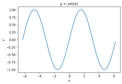
The “pyplot” module of matplotlib can be used in a similar way to Matlab, with repeated calls to plt.[...] updating the state of the figure being created:
import matplotlib.pyplot as plt
x = np.arange(-2*np.pi, 2*np.pi, 0.1)
y = np.sin(x)
plt.plot(x, y)
plt.xlabel("x")
plt.ylabel("y")
plt.title("y = sin(x)");

However, for full control of figures, it is more flexible to use the object oriented approach as below. For more, refer to the matplotlib tutorials
# Create a "figure" object that contains everything
fig = plt.figure()
# Add an "axes" object as part of the figure
ax = fig.add_subplot(111)
# NB: Instead of the above, it is more convenient to use:
#       fig, ax = plt.subplots(nrows=1, ncols=1)
# Add things to the axes
ax.plot(x, y)
ax.set_xlabel("x")
ax.set_ylabel("y")
ax.set_title("y = sin(x)");
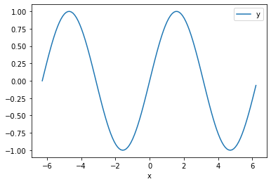
The demonstrations above show that there are quite a few lines of code necessary to do the typical data analysis flow of loading/generating data, performing some computation, and plotting the results, in addition to having to pass around variables (like x and y above). This code may very often be quite similar so you might imagine standardising this process. It is for this reason that pandas has become popular, which provides the DataFrame object (inspired by the R language). This enables us to create a single tabular object to pass around (called df below) that contains our data (in this case numpy arrays), that has built-in plotting methods to rapidly inspect the data (creating matplotlib figures). Pandas accepts a wide range of input formats to load data, and contains computational tools that are particularly useful for time series, as well as connecting to Dask for doing larger computations (larger than memory, multi-process, distributed etc.).
import pandas as pd
df = pd.DataFrame({"x": np.arange(-2*np.pi, 2*np.pi, 0.1),
                   "y": np.sin(np.arange(-2*np.pi, 2*np.pi, 0.1))})
df.head()
| x | y | |
|---|---|---|
| 0 | -6.283185 | 2.449294e-16 |
| 1 | -6.183185 | 9.983342e-02 |
| 2 | -6.083185 | 1.986693e-01 |
| 3 | -5.983185 | 2.955202e-01 |
| 4 | -5.883185 | 3.894183e-01 |
df.plot(x="x", y="y");
Moving beyond pandas, we come to xarray, which extends the pandas concepts to n-dimensional data.